
This tutorial introduces the Generalized Low Rank Model (GLRM) [1 ], a new machine learning approach for reconstructing missing values and identifying important features in heterogeneous data. It demonstrates how to build a GLRM in H2O that condenses categorical information into a numeric representation, which can then be used in other modeling frameworks such as deep learning .
What is a Low Rank Model?
Across business and research, analysts seek to understand large collections of data with numeric and categorical values. Many entries in this table may be noisy or even missing altogether. Low rank models facilitate the understanding of tabular data by producing a condensed vector representation for every row and column in the data set.
Specifically, given a data table A with m rows and n columns, a GLRM consists of a decomposition of A into numeric matrices X and Y. The matrix X has the same number of rows as A, but only a small, user-specified number of columns k. The matrix Y has k rows and d columns, where d is equal to the total dimension of the embedded features in A. For example, if A has 4 numeric columns and 1 categorical column with 3 distinct levels (e.g., red , blue and green ), then Y will have 7 columns. When A contains only numeric features, the number of columns in A and Y are identical, as shown below.

Both X and Y have practical interpretations. Each row of Y is an archetypal feature formed from the columns of A, and each row of X corresponds to a row of A projected into this reduced dimension feature space. We can approximately reconstruct A from the matrix product XY, which has rank k. The number k is chosen to be much less than both m and n: a typical value for 1 million rows and 2,000 columns of numeric data is k = 15. The smaller k is, the more compression we gain from our low rank representation.
GLRMs are an extension of well-known matrix factorization methods such as Principal Components Analysis (PCA). While PCA is limited to numeric data, GLRMs can handle mixed numeric, categorical, ordinal and Boolean data with an arbitrary number of missing values. It allows the user to apply regularization to X and Y, imposing restrictions like non-negativity appropriate to a particular data science context. Thus, it is an extremely flexible approach for analyzing and interpreting heterogeneous data sets.
Data Description
For this example, we will be using two data sets. The first is compliance actions carried out by the U.S. Labor Department’s Wage and Hour Division (WHD) from 2014-2015. This includes information on each investigation, including the zip code tabulation area (ZCTA) where the firm is located, number of violations found and civil penalties assessed. We want to predict whether a firm is a repeat and/or willful violator. In order to do this, we need to encode the categorical ZCTA column in a meaningful way. One common approach is to replace ZCTA with indicator variables for every unique level, but due to its high cardinality (there are over 32,000 ZCTAs!), this is slow and leads to overfitting.
Instead, we will build a GLRM to condense ZCTAs into a few numeric columns representing the demographics of that area. Our second data set is the 2009-2013 American Community Survey (ACS) 5-year estimates of household characteristics. Each row contains information for a unique ZCTA, such as average household size, number of children and education. By transforming the WHD data with our GLRM, we not only address the speed and overfitting issues, but also transfer knowledge between similar ZCTAs in our model.
Part 1: Condensing Categorical Data
Initialize the H2O server and import the ACS data set. We use all available cores on our computer and allocate a maximum of 2 GB of memory to H2O.
r

 library(h2o)

 h2o.init(nthreads = -1, max_mem_size = "2G")
We will need to set the path to a scratch directory that will contain the downloaded datasets. Please adjust at your will.
r

 workdir <- "/tmp"
Now, let’s import the ACS data into H2O and separate out the zip code tabulation area column.
r

 download.file("https://s3.amazonaws.com/h2o-public-test-data/bigdata/laptop/census/ACS_13_5YR_DP02_cleaned.zip", file.path(workdir, "ACS_13_5YR_DP02_cleaned.zip", "wget", quiet = TRUE))

 acs_orig <- h2o.importFile(path = file.path(workdir, "ACS_13_5YR_DP02_cleaned.zip"), col.types = c("enum", rep("numeric", 149)))

 acs_zcta_col <- acs_orig$ZCTA5

 acs_full <- acs_orig[,-which(colnames(acs_orig) == "ZCTA5")]
Get a summary of the ACS data set.
r

 dim(acs_full)

 summary(acs_full)
Build a GLRM to reduce ZCTA demographics to k = 10 archetypes. We standardize the data before model building to ensure a good fit. For the loss function, we select quadratic again, but this time, apply regularization to X and Y in order to sparsify the condensed features.
r
acs_model <- h2o.glrm(training_frame = acs_full, k = 10, transform = "STANDARDIZE", loss = "Quadratic", regularization_x = "Quadratic", regularization_y = "L1", max_iterations = 100, gamma_x = 0.25, gamma_y = 0.5)
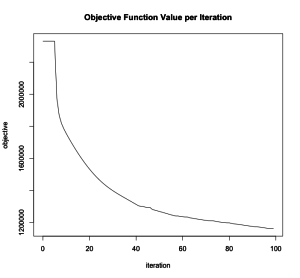
plot(acs_model)
From the plot of the objective function per iteration, we see that the algorithm has reached convergence.

The rows of the X matrix map each ZCTA into a combination of demographic archetypes.
r

 zcta_arch_x <- h2o.getFrame(acs_model@model$representation_name)

 head(zcta_arch_x)
Plot a few interesting ZCTAs on the first two archetypes. We should see cities with similar demographics, such as Sunnyvale and Cupertino, grouped close together, while very different cities, such as the rural town McCune and the upper east side of Manhattan, fall far apart on the graph.
r

 idx <- ((acs_zcta_col == "10065") | # Manhattan, NY (Upper East Side)

 (acs_zcta_col == "11219") | # Manhattan, NY (East Harlem)

 (acs_zcta_col == "66753") | # McCune, KS

 (acs_zcta_col == "84104") | # Salt Lake City, UT

 (acs_zcta_col == "94086") | # Sunnyvale, CA

 (acs_zcta_col == "95014")) # Cupertino, CA

 city_arch <- as.data.frame(zcta_arch_x[idx,1:2])

 xeps <- (max(city_arch[,1]) - min(city_arch[,1])) / 10

 yeps <- (max(city_arch[,2]) - min(city_arch[,2])) / 10

 xlims <- c(min(city_arch[,1]) - xeps, max(city_arch[,1]) + xeps)

 ylims <- c(min(city_arch[,2]) - yeps, max(city_arch[,2]) + yeps)

 plot(city_arch[,1], city_arch[,2], xlim = xlims, ylim = ylims, xlab = "First Archetype", ylab = "Second Archetype", main = "Archetype Representation of Zip Code Tabulation Areas")

 text(city_arch[,1], city_arch[,2], labels = c("Upper East Side", "East Harlem", "McCune", "Salt Lake City", "Sunnyvale", "Cupertino"), pos = 1)
![]()
Your plot may look different depending on how the GLRM algorithm was initialized. Try plotting other archetypes against each other, or re-run GLRM with rank k = 2 for the best two-dimensional representation of the ZCTAs.
Part 2: Runtime and Accuracy Comparison
We now build a deep learning model on the WHD data set to predict repeat and/or willful violators. For comparison purposes, we train our model using the original data, the data with the ZCTA column replaced by the compressed GLRM representation (the X matrix), and the data with the ZCTA column replaced by all the demographic features in the ACS data set.
Import the WHD data set and get a summary.
r

 download.file("https://s3.amazonaws.com/h2o-public-test-data/bigdata/laptop/census/whd_zcta_cleaned.zip", file.path(workdir, "whd_zcta_cleaned.zip", "wget", quiet = TRUE))

 whd_zcta <- h2o.importFile(path = file.path(workdir, "whd_zcta_cleaned.zip"), col.types = c(rep("enum", 7), rep("numeric", 97)))

 dim(whd_zcta)

 summary(whd_zcta)
Split the WHD data into test and train with a 20/80 ratio.
r

 split <- h2o.runif(whd_zcta)

 train <- whd_zcta[split <= 0.8,]

 test <- whd_zcta[split > 0.8,]
Build a deep learning model on the WHD data set to predict repeat/willful violators. Our response is a categorical column with four levels: N/A = neither repeat nor willful, R = repeat, W = willful, and RW = repeat and willful violator. Thus, we specify a multinomial distribution. We skip the first four columns, which consist of the case ID and location information that is already captured by the ZCTA.
r

 myY <- "flsa_repeat_violator"

 myX <- setdiff(5:ncol(train), which(colnames(train) == myY))

 orig_time <- system.time(dl_orig <- h2o.deeplearning(x = myX, y = myY, training_frame = train, validation_frame = test, distribution = "multinomial", epochs = 0.1, hidden = c(50,50,50)))
Replace each ZCTA in the WHD data with the row of the X matrix corresponding to its condensed demographic representation. In the end, our single categorical column will be replaced by k = 10 numeric columns.
r

 zcta_arch_x$zcta5_cd <- acs_zcta_col

 whd_arch <- h2o.merge(whd_zcta, zcta_arch_x, all.x = TRUE, all.y = FALSE)

 whd_arch$zcta5_cd <- NULL

 summary(whd_arch)
Split the reduced WHD data into test/train and build a deep learning model to predict repeat/willful violators.
r

 train_mod <- whd_arch[split <= 0.8,]

 test_mod <- whd_arch[split > 0.8,]

 myX <- setdiff(5:ncol(train_mod), which(colnames(train_mod) == myY))

 mod_time <- system.time(dl_mod <- h2o.deeplearning(x = myX, y = myY, training_frame = train_mod, validation_frame = test_mod, distribution = "multinomial", epochs = 0.1, hidden = c(50,50,50)))
Replace each ZCTA in the WHD data with the row of ACS data containing its full demographic information.
r

 colnames(acs_orig)[1] <- "zcta5_cd"

 whd_acs <- h2o.merge(whd_zcta, acs_orig, all.x = TRUE, all.y = FALSE)

 whd_acs$zcta5_cd <- NULL

 summary(whd_acs)
Split the combined WHD-ACS data into test/train and build a deep learning model to predict repeat/willful violators.
r

 train_comb <- whd_acs[split <= 0.8,]

 test_comb <- whd_acs[split > 0.8,]

 myX <- setdiff(5:ncol(train_comb), which(colnames(train_comb) == myY))

 comb_time <- system.time(dl_comb <- h2o.deeplearning(x = myX, y = myY, training_frame = train_comb, validation_frame = test_comb, distribution = "multinomial", epochs = 0.1, hidden = c(50,50,50)))
Compare the performance between the three models. We see that the model built on the reduced WHD data set finishes almost 10 times faster than the model using the original data set, and it yields a lower log-loss error. The model with the combined WHD-ACS data set does not improve significantly on this error. We can conclude that our GLRM compressed the ZCTA demographics with little informational loss.
r

 data.frame(original = c(orig_time[3], h2o.logloss(dl_orig, train = TRUE), h2o.logloss(dl_orig, valid = TRUE)),

 reduced = c(mod_time[3], h2o.logloss(dl_mod, train = TRUE), h2o.logloss(dl_mod, valid = TRUE)),

 combined = c(comb_time[3], h2o.logloss(dl_comb, train = TRUE), h2o.logloss(dl_comb, valid = TRUE)),

 row.names = c("runtime", "train_logloss", "test_logloss"))

 # original reduced combined

 # runtime 40.3590000 6.5790000 7.5500000

 # train_logloss 0.2467982 0.1895277 0.2440147

 # test_logloss 0.2429517 0.1980886 0.2277701
References
- M. Udell, C. Horn, R. Zadeh, S. Boyd (2014). Generalized Low Rank Models. Unpublished manuscript, Stanford Electrical Engineering Department. http://arxiv.org/abs/1410.0342