

If you can’t explain it to a six-year-old, you don’t understand it yourself. – Albert Einstein
One fear caused by machine learning (ML) models is that they are blackboxes that cannot be explained. Some are so complex that no one, not even domain experts, can understand why they make certain decisions. This is of particular concern when such models are used to make high-stakes decisions like determining if someone should be released from prison or giving a patient a risky surgical procedure.
The field of Explainable or Interpretable ML (often denoted XML) focuses on creating tools and methods to describe how ML models make decisions. One fundamental technique in this domain is Shapley values, and in this article, we provide a gentle introduction to what they are and how you can use them.
Shapley Values – An Intuitive Explanation
Let’s say we are a farming collective and have made $1 million profit this year. How do we share this sum?
We could give each member an equal share. But what if one member contributed to 80% of the sales? What if the money is sitting in one member’s bank account, and they say they will give it all to charity unless they get a fair share? What if one member didn’t make any sales but provided machinery that increased everyone’s productivity and thus increased sales by 20%?
Each member contributes in different ways, and it’s not straightforward to decide how much money each member should receive. Shapley values are the method Lloyd Shapley proposed back in 1951 to solve this problem and give each member a fair share.
Shapley was studying cooperative game theory when he created this tool. However, it is easy to transfer it to the realm of machine learning. We simply treat a model’s prediction as the ‘surplus’ and each feature as a ‘farmer in the collective.’ The Shapley value tells us how much impact each element has on the prediction, or (more precisely) how much each feature moves the prediction away from the average prediction.
Calculating Shapley Values
Here are the steps to calculate the Shapley value for a single feature F:
- Create the set of all possible feature combinations (called coalitions)
- Calculate the average model prediction
- For each coalition, calculate the difference between the model’s prediction without F and the average prediction.
- For each coalition, calculate the difference between the model’s prediction with F and the average prediction.
- For each coalition, calculate how much F changed the model’s prediction from the average (i.e., step 4 – step 3) – this is the marginal contribution of F.
- Shapley value = the average of all the values calculated in step 5 (i.e., the average of F’s marginal contributions)
In short, the Shapley value of a feature F is the average marginal contribution F provides the model across all possible coalitions.
To keep it simple, we are avoiding rigorous mathematical definitions, but if you want them, head over to Wikipedia or the excellent free book Interpretable Machine Learning by Christoph Molnar.
If you think this is a lot to calculate, you’d be right. With K total features, there are 2**K coalitions and thus, calculating Shapley values scales exponentially! This property made it difficult to work with them for decades. But recently, there was a breakthrough.
Shapley Values in Python
In 2017, Lundberg and Lee published a paper titled A Unified Approach to Interpreting Model Predictions . They combined Shapley values with several other model explanation methods to create SHAP values (SHapley Additive exPlanations) and the corresponding shap library.
If you want to create Shapley values for your model, chances are you will actually generate SHAP values – indeed, in our research, we couldn’t find a library implementing Shapley values. This is great as SHAP takes all the benefits of Shapley values and improves upon many negatives. We save an in-depth analysis of the shap library for a future article but want to share some useful visualizations with you to whet your appetite.
We will use a subset of the Wine Rating & Price dataset from Kaggle. This dataset contains five csv files, but we will only work with Red.csv, roughly 8,500 rows. It contains data scraped from Vivino.com, the world’s largest wine marketplace. Each wine on the site has a rating to help inform your purchase decision. We will use a sample of feature columns to predict each wine’s rating (out of 5) and inspect the Shapley values using the shap library.
# Standard imports
import pandas as pd
import numpy as np
import matplotlib.pyplot as plt
import seaborn as sns
# Import shap and our model
import shap
from lightgbm import LGBMRegressor
# Nicest style for SHAP plots
sns.set(style='ticks')
First, we load the libraries we need. We use LightGBM, but you can use any regressor you want.
red = pd.read_csv('Red.csv')
# Drop the 8 rows that are Non-Vintage i.e. NaNs
non_vintage = red.Year == 'N.V.'
red = red.drop(red[non_vintage].index, axis=0)
# Just keep numeric columns
X = red[['Price', 'Year', 'NumberOfRatings']]
# Cast all columns to numeric type
X = X.apply(pd.to_numeric)
y = red.Rating
We read in our csv file, drop the 8 NaN rows, create X from the numeric columns, and y as the Rating column.
Price is the price of the wine in Euros, Year is the year the wine was produced, and NumberOfRatings is the number of people who have rated this wine already.
# Create and fit model
model = LGBMRegressor()
model.fit(X, y)
Then we instantiate and fit our LightGBM regressor (this takes less than two seconds, even on CPU).
# Create Explainer and get shap_values
explainer = shap.Explainer(model, X)
shap_values = explainer(X)
Next, we create an Explainer object, and from that, we get the SHAP values.
print(shap_values.shape) # (8658, 3)
print(shap_values.shape == X.shape) # True
print(type(shap_values)) # <class 'shap._explanation.Explanation'>
The shap_values object is the same shape as X and is an Explanation object.
print(shap_values[1])
.values = array([-0.13709112, 0.04292881, 0.01909666])
.base_values = 3.892730293342654
.data = array([ 15.5, 2017. , 100. ])
Looking at the contents of index 1 of shap_values, we see it contains:
-
.values– the SHAP values themselves, .base_values– the average prediction for our model, and.data– the original X data
You can access each of these individually with the dot notation accessor should you desire. Thankfully, most shap plots accept Explanation objects and do the heavy lifting for you in the background.
Let’s make some waterfall plots.
shap.plots.waterfall(shap_values[1])
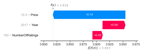
Waterfall plots show how the SHAP values move the model prediction from the expected value E[f(X)] displayed at the bottom of the chart to the predicted value f(x) at the top. They are sorted with the smallest SHAP values at the bottom.
The expected value 3.893 given by shap_values.base_values is at the bottom of the plot. The original X data given by shap_values.data indicates the features and their corresponding values on the left-hand side. Finally, SHAP values given by shap_values.values are displayed as red or blue arrows depending on whether they increase or decrease the predicted value.
We see that NumberOfRatings = 100 and Year = 2017 have a positive impact on this wine with a net gain of 0.02 + 0.04 = 0.06. However, Price = €15.50 decreases the predicted rating by 0.14. So, this wine has a predicted rating of 3.893 + 0.02 + 0.04 – 0.14 = 3.818, which you can see at the top of the plot. By summing the SHAP values, we calculate this wine has a rating 0.02 + 0.04 – 0.14 = -0.08 below the average prediction. Adding SHAP values together is one of their key properties and is one reason they are called Shapley additive explanations.
Let’s look at another example.
shap.plots.waterfall(shap_values[14])
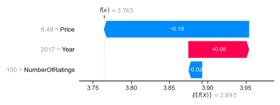
This wine also has NumberOfRatings = 100 and Year = 2017, but it has different SHAP values. In the first plot, NumberOfRatings = 100 resulted in +0.02, but for this plot, it is -0.02. In the first plot, Year = 2017 gave +0.04, but in this plot, it is +0.08. This disparity demonstrates that even if samples have the same values for certain features, it does not guarantee they have the same SHAP values. Explaining the reasoning for this is out of scope for this article but being aware is enough for now.
Finally, let’s look at a feature importance style plot commonly seen with tree-based models.
shap.plots.bar(shap_values)
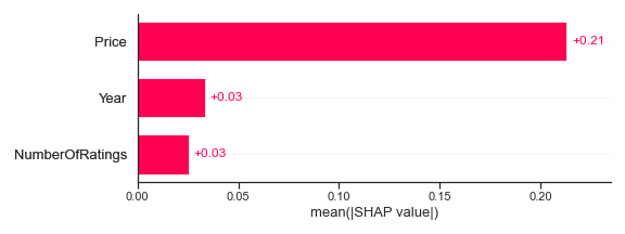
We’ve plotted the mean SHAP value for each of the features. Price is the highest with an average of +0.21, while Year and NumberOfRatings are similar at +0.03 each. Therefore, a higher value for each feature generally increases the predicted rating.
Shapley Values and H2O
At H2O, we’ve baked Shapley/SHAP values and other world-class model interpretability methods into both AI Hybrid Cloud (through Driverless AI ) and H2O-3 . For example, in Driverless AI, you can compare the Shapley values for your original features against the Shapley values for the transformed features. This technique is helpful if you are doing heavy feature engineering and want to know the difference in predictive power between the two sets.
Conclusion
Shapley values were created over 70 years ago to ensure a fair payout in cooperative games. Now the machine learning community has taken them on board and uses them to interpret models in a theoretically sound way. We covered the tip of the iceberg for this potent and valuable tool. We hope this article has given you the courage to start using Shapley and SHAP values to transform your blackbox models into glassboxes that you can deeply understand and use to create massive positive change in the world.
If you want to quickly build world-class models and interpret them with Shapley values in just a few clicks, request a demo of H2O’s AI Cloud today.