This document gives guidelines for performance tuning of H2O Deep Learning, both in terms of speed and accuracy. It is intended for existing users of H2O Deep Learning (which is easy to change if you’re not), as it assumes some familiarity with the parameters and use cases.

Motivation

This effort was in part motivated by a Deep Learning project that benchmarked against H2O, and we tried to reproduce their results, especially since they claimed that H2O is slower.

Summary of our findings (much more at the end of part 1):
* We are unable to reproduce their findings (our numbers are 9x to 52x faster, on a single node)
* The benchmark was only on raw training throughput and didn’t consider model accuracy (at all)
* We present improved parameter options for higher training speed (more below)
* We present a single-node model that trains faster than their 16-node system (and leads to higher accuracy than with their settings)

More Information!

Please consult the H2O documentation, H2O World Training and the H2O Booklets for detailed instructions on H2O and H2O Deep Learning. There are many YouTube videos and Slide decks on H2O Deep Learning. You can also follow me on @ArnoCandel to stay up-to-date. Don’t forget to read the KDNuggets interview, which covers a lot of the ideas and use cases for H2O and H2O Deep Learning in particular. This tutorial does not attempt to explain the many potential hyper-parameters of H2O Deep Learning.

Getting Started

To reproduce these results (up to small numerical noise intrinsic to the underlying methods), you can download and execute this script (here’s the raw version). It will download H2O, launch a single-node H2O cluster on your laptop or workstation and run the benchmarks. The script is both valid R and markdown code, and should run out of the box for you in RStudio (download, open in RStudio, install rmarkdown package, then click on Chunks -> Run All). It was also used to create this blog via a simple bash script. Please contact me if you have questions or comments.
The full logs of the run that created this blog post are available for download here. Note: results updated as of March 4 (now on Windows 8.1, system wasn’t overclocked in previous post)

options(repos=structure(c(CRAN='http://cran.us.r-project.org')))
install.packages("rmarkdown")

Distributed Benchmarking – Coming Soon

As many of you might know, distributed benchmarking has its own issues and complexity. I’ve burned many millions of core hours on the world’s fastest supercomputers over the last decade, so I have a good sense of what it takes to get code to scale. Interconnect performance, load balancing and algorithmic choices greatly affect the scalability of large distributed systems. This benchmark script can seamlessly run on a large multi-node H2O cluster (where some parameters would benefit from some changes), and the scalability of H2O Deep Learning can be fully tuned from close-to-linear speedup with very little communication to totally communication-dominated regimes. The current implementation automatically attempts to balance computation and communication with dynamic auto-tuning during runtime.
Due to the complexity involved, we refer to a later blog on distributed benchmarking of H2O Deep Learning, so please stay tuned for that. We will, however, show some existing use cases and a prior scaling study on multi-node configurations, as practically all our applications of H2O Deep Learning in-house and by customers are run in distributed mode.

Part 1 – Single-Node Training Speed

For simplicity, we start with some single-node experiments quantifying the raw training speed. Of course, many of the parameters we’ll change affect the predictive accuracy of a model, but for this first part, and to get an idea of how H2O Deep Learning works, we only look at the raw training speed (number of processed training samples per second).

Establish Connection to H2O

For this study, we use the latest version of H2O, h2o-dev. The numerical performance of H2O Deep Learning in h2o-dev is very similar to the performance of its equivalent in h2o. Instructions for installation and execution in stand-alone mode, R, Python, Hadoop or Spark environments can be found at h2o.ai/download, but you can just follow this script from R, and everything should just work.
We use nightly build 1079 of h2o-dev, but you should be able to use any future nightly or stable version as well. The code below is copied from the instructions from the h2o download page.
The following two commands remove any previously installed H2O packages for R.

if ("package:h2o" %in% search()) { detach("package:h2o", unload=TRUE) }
if ("h2o" %in% rownames(installed.packages())) { remove.packages("h2o") }

Next, we download packages that H2O depends on.

if (! ("methods" %in% rownames(installed.packages()))) { install.packages("methods") }
if (! ("statmod" %in% rownames(installed.packages()))) { install.packages("statmod") }
if (! ("stats" %in% rownames(installed.packages()))) { install.packages("stats") }
if (! ("graphics" %in% rownames(installed.packages()))) { install.packages("graphics") }
if (! ("RCurl" %in% rownames(installed.packages()))) { install.packages("RCurl") }
if (! ("rjson" %in% rownames(installed.packages()))) { install.packages("rjson") }
if (! ("tools" %in% rownames(installed.packages()))) { install.packages("tools") }
if (! ("utils" %in% rownames(installed.packages()))) { install.packages("utils") }

Now we download, install and initialize the H2O package for R.

install.packages("h2o", type="source", repos=(c("http://h2o-release.s3.amazonaws.com/h2o-dev/master/1079/R")))
library(h2o)
library('stringr')

Start a single-node instance of H2O using all available processor cores and reserve 4GB of memory (less should work too, check your logs for WARN: Pausing to swap to disk; more memory may help using the Flow GUI at localhost:54321, Admin -> View Log -> SELECT LOG FILE TYPE: warn).

h2oServer <- h2o.init(ip="localhost", port=54321, max_mem_size="4g", nthreads=-1)
#h2oServer <- h2o.init(ip="h2o-cluster", port=54321) # optional: connect to running H2O cluster

We will need to set the path to a scratch directory that will contain the downloaded datasets and the CSV files containing the results. Please adjust at your will.

workdir="/tmp"

Load Benchmark Dataset into H2O’s Memory

Next, we download the well-known MNIST dataset of hand-written digits, where each row contains the 28^2=784 gray-scale pixel values from 0 to 255 of digitized digits (last column contains labels from 0 to 9). The training and testing datasets are also available at H2O Github. The training dataset has 60,000 rows and the test set has 10,000 rows.
We are well aware that this is small data for today’s standards, but since H2O Deep Learning is a fully distributed streaming algorithm that processes point-by-point, its performance in terms of throughput will remain similar for much larger datasets as each processor core streams through training samples (i.e., image, data point, row) one at a time. The maximum dataset size that can be handled is given by the total aggregate amount of memory of all nodes and the compression ratio of the dataset (H2O does lossless compression).
We upload the MNIST datasets (train and test sets) into H2O’s memory. Keep in mind that R just serves as a remote control for this entire experiment and never does any actual computation. All the heavy lifting is done by the fully parallelized H2O in-memory engine.

download.file("https://s3.amazonaws.com/h2o-training/mnist/train.csv.gz",
file.path(workdir,"train.csv.gz"), "wget", quiet = T)
download.file("https://s3.amazonaws.com/h2o-training/mnist/test.csv.gz",
file.path(workdir,"test.csv.gz"), "wget", quiet = T)
train_hex <- h2o.importFile(h2oServer, path = file.path(workdir,"train.csv.gz"),
header = F, sep = ',', key = 'train.hex')
test_hex <- h2o.importFile(h2oServer, path = file.path(workdir,"test.csv.gz"),
header = F, sep = ',', key = 'test.hex')

Performance Metrics and Observables

In this first part of the benchmark study, we will investigate the single-node performance of H2O Deep Learning in terms of training examples per second, mostly ignoring the test set error except for some notable occasions.
Notes:

• For each set of parameters (in addition to specifying the training data, and the predictors and response column), we run H2O Deep Learning and record training samples, training time, training speed, and test set error.
• The clock starts at the moment the first training example is presented to the neural network, and stops when model building is done. The stopping criterion is the number of epochs (i.e., the number of training samples relative to the training data set size). Training speed is computed as the number of training samples seen since the clock was started, divided by the seconds that have passed. We note that the raw processing speed is somewhat underestimated by this (conservative) approach, as anything that is not training such as scoring or computing statistics counts towards the total time.
• The classification error on the entire test set (10,000 rows) is computed after training is done, for all runs. The time for this is not counted.
• H2O Deep Learning uses online learning with stochastic gradient descent and back-propagation. There are no mini-batches (or only trivial ones of size 1), every training sample immediately affects the network weights for fastest convergence and highest model accuracy.
• Intentional race conditions between multiple threads a la Hogwild! avoid locking, but lead to non-reproducible results, unless reproducible=T is specified and a seed is given (which then runs on 1 core – not done here).
• Hardware specs: Intel i7 5820k (6 cores @4.4GHz). Yes, it’s an overclocked sub-$400 processor. If it dies, I’ll have to get the 8-core version…
• It is possible to run individual pieces (code Chunks) or the entire script at once, each benchmark has its own CSV results file.

Here we go. First, we set up some helper function to run H2O Deep Learning with user-given parameters, and to write the parameters and observables to CSV files.

score_test_set=T #disable if only interested in training throughput
run <- function(extra_params) {
str(extra_params)
print("Training.")
model <- do.call(h2o.deeplearning, modifyList(list(x=1:784, y=785, do_classification=T,
training_frame=train_hex, destination_key="dlmodel"), extra_params))
sampleshist <- model@model$scoringHistory$"Training Samples"
samples <- sampleshist[length(sampleshist)]
time <- model@model$run_time/1000
print(paste0("training samples: ", samples))
print(paste0("training time : ", time, " seconds"))
print(paste0("training speed : ", samples/time, " samples/second"))
if (score_test_set) {
print("Scoring on test set.")
## Note: This scores full test set (10,000 rows) - can take time!
test_error <- h2o.performance(model, test_hex)@metrics$cm$prediction_error
print(paste0("test set error : ", test_error))
} else {
test_error <- 1.0
}
h2o.rm("dlmodel")
c(paste(names(extra_params), extra_params, sep = "=", collapse=" "),
samples, sprintf("%.3f", time),
sprintf("%.3f", samples/time), sprintf("%.3f", test_error))
}
writecsv <- function(results, file) {
table <- matrix(unlist(results), ncol = 5, byrow = TRUE)
colnames(table) <- c("parameters", "training samples",
"training time", "training speed", "test set error")
write.csv(table, file.path(workdir,file),
col.names = T, row.names=F, quote=T, sep=",")
}

First Study – Various Neural Network Topologies

As a first study, we vary the network topology, and we also fix a number of training samples, specified by the number of epochs (we process approximately 10% of the dataset here, chosen at random). All other parameters are left at default values (per-weight adaptive learning rate, no L1/L2 regularization, no Dropout, Rectifier activation function). Note that we run shallow neural nets (1 hidden layer), and deep neural nets with 2 or 3 hidden layers. You can modify this and run other parameter combinations as well (and the same holds for all experiments here).
The number of columns of the dataset (all numerical) translates directly into the size of the first layer of neurons (input layer), and hence significantly affects the size of the model. The number of output neurons is 10, one for each class (digit) probability. For the MNIST dataset, all Deep Learning models below will have 717 input neurons, as the other 67 pixel values are constant (white background) and thus ignored. The size of the model is given by the number of connections between the fully connected input+hidden+output neuron layers (and their bias values), and grows as the sum of the product of the number of connected neurons (~quadratically). Since training involves reading and updating all the model coefficients (weights and biases), the model complexity is linear in the size of the model, up to memory hierarchy effects in the x86 hardware. The speed of the memory subsystem (both in terms of latency and bandwidth) has a direct impact on training speed.

EPOCHS=.1 #increase if you have the patience (or run multi-node), shouldn't matter much for single-node
args <- list(
list(hidden=c(64), epochs=EPOCHS),
list(hidden=c(128), epochs=EPOCHS),
list(hidden=c(256), epochs=EPOCHS),
list(hidden=c(512), epochs=EPOCHS),
list(hidden=c(1024), epochs=EPOCHS),
list(hidden=c(64,64), epochs=EPOCHS),
list(hidden=c(128,128), epochs=EPOCHS),
list(hidden=c(256,256), epochs=EPOCHS),
list(hidden=c(512,512), epochs=EPOCHS),
list(hidden=c(1024,1024), epochs=EPOCHS),
list(hidden=c(64,64,64), epochs=EPOCHS),
list(hidden=c(128,128,128), epochs=EPOCHS),
list(hidden=c(256,256,256), epochs=EPOCHS),
list(hidden=c(512,512,512), epochs=EPOCHS),
list(hidden=c(1024,1024,1024), epochs=EPOCHS)
)
writecsv(lapply(args, run), "network_topology.csv")

We can plot the training speed (x-axis, more is faster) for the runs above, in the same order as the listing above. On the y-axis, we denote the overall training time in seconds.

As expected, smaller and shallower networks run faster, and larger, deeper networks take more time. An interesting exception is the smallest network (717->64->10 neurons), which has only 717*64 + 64*10 + 64 + 10 = 46602 model parameters (plus adaptive learning rate overhead of a factor of 2), but something prevents this from running faster (unclear, need to look into it, probably cache trashing). You can confirm the network topology and model size (among other useful things) by inspecting the logs (available via the Flow GUI on localhost:54321), and the output will look similar to this:

# Number of model parameters (weights/biases): 46,602
# ...
# Number of hidden layers is 1
# Status of Neuron Layers:
# # Units Type Dropout L1 L2 Rate (Mean,RMS) Weight (Mean,RMS) Bias (Mean,RMS)
# 1 717 Input 0.00 %
# 2 64 Rectifier 0.00 % 0.0000 0.0000 (0.0000, 0.0000) (0.0000, 0.0000) (0.0000, 0.0000)
# 3 10 Softmax 0.0000 0.0000 (0.0000, 0.0000) (0.0000, 0.0000) (0.0000, 0.0000)

For your convenience, here’s the raw data from the CSV file network_topology.csv in directory work_dir:

Scoring Overhead

During training, the model is getting scored on both the training and optional validation datasets at user-given intervals, with a user-given duty cycle (fraction of training time) and on user-specified subsamples of the datasets. Sampling can help reduce this scoring overhead significantly, especially for large network topologies. Often, a statistical scoring uncertainty of 1% is good enough to get a sense of model performance, and 10,000 samples are typically fine for that purpose. For multi-class problems, score_validation_sampling can be set to stratified sampling to maintain a reasonable class representation.
For small networks and small datasets, the scoring time is usually negligible. The training data set is sub-sampled to score_training_samples (default: 10,000) rows (for use in scoring only), while a user-given validation dataset is used in full, without sampling (score_validation_samples=0) unless specified otherwise. This is important to understand, as it can lead to a large scoring overhead, especially for short overall training durations (no matter how few samples are trained), as scoring happens at least once (every score_interval (default: 5) seconds after the first MapReduce pass is complete, and at least once at the end of training), but no more than a duty_cycle (default: 10%) fraction of the total runtime.
To illustrate this, we train the same model 7 times with different scoring selections.

args <- list(
list(hidden=c(1024, 1024), epochs=EPOCHS, validation_frame=test_hex),
list(hidden=c(1024, 1024), epochs=EPOCHS, score_training_samples=60000,
score_duty_cycle=1, score_interval=1),
list(hidden=c(1024, 1024), epochs=EPOCHS, score_training_samples=60000),
list(hidden=c(1024, 1024), epochs=EPOCHS, score_training_samples=10000),
list(hidden=c(1024, 1024), epochs=EPOCHS, score_training_samples=1000),
list(hidden=c(1024, 1024), epochs=EPOCHS, score_training_samples=100),
list(hidden=c(1024, 1024), epochs=EPOCHS, score_training_samples=100,
score_duty_cycle=0, score_interval=10000)
)
writecsv(lapply(args, run), “scoring_overhead.csv”)

As you can see, the overhead for scoring the entire training dataset at every opportunity (after each MapReduce pass, more on this below) can be significant (it’s the same as forward propagation!). The default option (first run) with a specified (reasonably sized) validation dataset is a good compromise, and it’s further possible to reduce scoring to a minimum. Test set classification errors are computed after training is finished, and are expected to be similar here (same model parameters) up to noise due to different initial conditions and (intentional) multi-threading race conditions (see Hogwild! reference above).

Adaptive vs Manual Learning Rate and Momentum

Next, we compare adaptive (per-coefficient) learning rate versus manually specifying learning rate and optional momentum.

args <- list(
list(hidden=c(1024, 1024), epochs=EPOCHS,
score_training_samples=100, adaptive_rate=T),
list(hidden=c(1024, 1024), epochs=EPOCHS,
score_training_samples=100, adaptive_rate=T,
rho=0.95, epsilon=1e-6),
list(hidden=c(1024, 1024), epochs=EPOCHS,
score_training_samples=100, adaptive_rate=F),
list(hidden=c(1024, 1024), epochs=EPOCHS,
score_training_samples=100, adaptive_rate=F,
rate=1e-3, momentum_start=0.5, momentum_ramp=1e5, momentum_stable=0.99)
)
writecsv(lapply(args, run), "adaptive_rate.csv")

It is clear that the fastest option is to run with a manual learning rate and without momentum (default: 0), as this reduces the memory and computational overhead to a minimum. Enabling the adaptive learning rate is roughly equivalent to turning on momentum training (as each model coefficient keeps track of its history), it is only slightly more computationally expensive (it uses an approximate square-root function that only costs a few clock cycles). Also, different hyper-parameters for adaptive learning rate can affect the training speed (at least for Rectifier activation functions, where back-propagation depends on the activation values).
Note that the lowest test set error was achieved with default settings (adaptive learning rate), corroborating our approach. For cases where fastest model training is required (possibly at the expense of highest achievable accuracy), manual learning rates without momentum can be a good option, but in general, adaptive learning rate simplifies the usage of H2O Deep Learning and make this tool highly usable by non-experts.

Training Samples Per Iteration

As explained earlier, model scoring (and multi-node model averaging) happens after every MapReduce step, the length of which is given in terms of the number of training samples via the parameters train_samples_per_iteration. It can be set to any value, -2, -1, 0, 1, 2, … and as high as desired. Special values are -2 (auto-tuning), -1 (all available data on each node) and 0 (one epoch). Values of 1 and above specify the (approximate) number of samples to process per MapReduce iteration. If the value is less than the number of training data points per node, stochastic sampling without replacement is done on the node-local data (which can be the entire dataset if replicate_training_data=T). If the value is larger than the number of training data points per node, stochastic sampling with replacement is done on the node-local data. In either case, the number of actually processed samples can vary between runs due to the stochastic nature of sampling. In single-node operation, there is potentially some model scoring overhead in-between these MapReduce iterations (see above for dependency on parameters), but no model-averaging overhead as there is only one model per node (racily updated by multiple threads).

args <- list(
list(hidden=c(1024, 1024), epochs=EPOCHS, score_training_samples=100,
score_interval=1, train_samples_per_iteration=-2),
list(hidden=c(1024, 1024), epochs=EPOCHS, score_training_samples=100,
score_interval=1, train_samples_per_iteration=100),
list(hidden=c(1024, 1024), epochs=EPOCHS, score_training_samples=100,
score_interval=1, train_samples_per_iteration=1000),
list(hidden=c(1024, 1024), epochs=EPOCHS, score_training_samples=100,
score_interval=1, train_samples_per_iteration=6000)
)
writecsv(lapply(args, run), "train_samples_per_iteration.csv")

As expected, the difference in the speed of the runs above is (for single-node operation) dominated by the frequency of model scoring, and the default settings (train_samples_per_iteration=-2, auto-tuning) is a reasonable compromise. This parameter will become much more important in multi-node operation where network communication affects both model accuracy and training speed (somewhat inversely). We also note that the test set error can fluctuate a bit as the sampling is non-deterministic (unless a seed is specified and reproducible=T).

Different activation functions

The activation function can make a big difference in runtime, as evidenced below. The reason for this is that H2O Deep Learning is optimized to take advantage of sparse activation of the neurons, and the Rectifier activation function (max(0,x)) is sparse and leads to less computation (at the expense of some accuracy, for which the speed often more than compensates for). Dropout (default: 0.5, randomly disable half of the hidden neuron activations for each training row) further increases the sparsity and makes training faster, and for noisy high-dimensional data, often also leads to better generalization (lower test set error) as it is a form of ensembling of many models with different network architectures. Since Dropout is a choice the user needs to make (at least for now), our default Rectifier activation function seems like a reasonable choice, especially since it also leads to a low test set error. We note that we omitted the Maxout activation here as we find it least useful (might require a revisit).

args <- list(
list(hidden=c(1024, 1024), epochs=EPOCHS, score_training_samples=100,
train_samples_per_iteration=1000, activation=”Rectifier”),
<p>list(hidden=c(1024, 1024), epochs=EPOCHS, score_training_samples=100,
train_samples_per_iteration=1000, activation=”RectifierWithDropout”),
<p>list(hidden=c(1024, 1024), epochs=EPOCHS, score_training_samples=100,
train_samples_per_iteration=1000, activation=”Tanh”),
<p>list(hidden=c(1024, 1024), epochs=EPOCHS, score_training_samples=100,
train_samples_per_iteration=1000, activation=”TanhWithDropout”)
)
writecsv(lapply(args, run), “activation_function.csv”)

External Large Deep Network Benchmark

Recently, we learned of a Deep Learning project that benchmarked against H2O, and we tried to reproduce their results, especially since they claimed that H2O is slower.
Since we know that all the compute cores are 100% max’ed out with H2O Deep Learning, or, as my colleagues call it, They got Arno’d… I had to see what’s going on. And trust me, I have profiled the living daylight out of H2O Deep Learning, and added some low-level optimizations for maximum throughput.
For a direct comparison, we aim to use the same H2O parameters as the external H2O Benchmark study (which was using Java and Scala code instead of R, but that doesn’t make a difference in runtime, as the same H2O Java code is executed):

# DeepLearningParameters dlParams = new DeepLearningParameters();
# dlParams._train = train_frame._key;
# dlParams._valid = test_frame._key;
# dlParams._response_column = "C785";
# dlParams._replicate_training_data = false;
# dlParams._epochs = 1;
# dlParams._hidden = new int[] {2500,2000,1500,1000,500,10};
# dlParams._activation = Activation.Tanh;
# dlParams._train_samples_per_iteration = 1500*NODES;
# DeepLearning dl = new DeepLearning(dlParams);
# dl.trainModel().get();

Notes:

• Unfortunately, there was no attempt made at comparing test set errors in the benchmark study. Throughput alone is not a good measure of model performance, see part 2 below for test set error comparisons and our model with world-record test set accuracy on the MNIST dataset.
• From the parameters used by the benchmark study, we can see that the Java field _convert_to_enum was left at its default value of false, leading to a regression model (1 output neuron with MeanSquare loss function), which is arguably not the best way to do digit classification. We will set the corresponding parameter in R with do_classification=T.
• We also note that the last hidden layer was specified to have 10 neurons, probably with the intention to emulate the 10-class probability distribution in the last hidden layer of 10 deep features. However, in H2O, the output layer is automatically added after the last hidden layer, and the user only specifies the hidden layers. For correctness, we will keep the first 5 hidden layers, and let H2O Deep Learning add the output layer with 10 neurons (and the CrossEntropy loss function) automatically (since we’re also setting do_classification=T). We note that the difference in model size (and loss function) is a mere 11 numbers, and has no impact on training speed (final layers 500->10->1 vs 500->10).
• For unknown reasons, the benchmarkers instrumented the H2O .jar file to measure speed inside the mappers/reducers. This is neither necessary nor very useful, as the logs already print out the training speed based on pure wall clock time, which is easily verified.
• H2O Deep Learning currently only does online learning (mini-batch size of 1), while it appears that the other method used a mini-batch size of 1000. This algorithmic difference both affects computational performance and model accuracy, and makes comparisons between different mini-batch sizes less useful (but still interesting).
• Given our observations above, parameters such as the scoring overhead or the choice of activation function has to be considered carefully, especially since the model has over 12 million weights and scoring (forward propagation) is going to take a significant amount of time even on the validation frame with “only” 10,000 rows.
• A large part of the benchmark study was concerned with the distributed scalability (strong scaling) of H2O (at least in terms of throughput). We will address this topic in part 3, but as noted earlier, almost linear speedups can be achieved when adding compute nodes as the communication overhead is fully user-controllable.
• For our single-node comparison (NODES=1), the parameter replicate_training_data has no effect, so we can leave it at its default value (TRUE).

We first run with the same parameters as the benchmark study, and then modify the parameters to improve the training speed successively.

#score_test_set=F ## uncomment if test set error is not needed<br />
EPOCHS=1
args <- list(<br />
list(hidden=c(2500,2000,1500,1000,500), epochs=EPOCHS, activation=”Tanh”,<br />
train_samples_per_iteration=1500, validation_frame=test_hex),</p>
<p>list(hidden=c(2500,2000,1500,1000,500), epochs=EPOCHS, activation=”Tanh”,<br />
train_samples_per_iteration=1500,<br />
score_training_samples=100, score_duty_cycle=0),</p>
<p>list(hidden=c(2500,2000,1500,1000,500), epochs=EPOCHS, activation=”Tanh”,<br />
train_samples_per_iteration=1500, adaptive_rate=F,<br />
score_training_samples=100, score_duty_cycle=0),</p>
<p>list(hidden=c(2500,2000,1500,1000,500), epochs=EPOCHS, activation=”Rectifier”,<br />
train_samples_per_iteration=1500, max_w2=10,<br />
score_training_samples=100, score_duty_cycle=0),</p>
<p>list(hidden=c(2500,2000,1500,1000,500), epochs=EPOCHS, activation=”RectifierWithDropout”,<br />
train_samples_per_iteration=1500, adaptive_rate=F, max_w2=10,<br />
score_training_samples=100, score_duty_cycle=0)<br />
)<br />
writecsv(lapply(args, run), “large_deep_net.csv”)<br />

Observations:
* We cannot reproduce the slow performance (~10 samples per second) cited by the other benchmark study. Using the same parameters, we measure a training speed of 91 samples per second on a single i7 5820k consumer PC.
* When removing the scoring overhead by not specifying validation_frame and reducing the score_training_samples to 100 (while keeping the Tanh activation and adaptive_rate=T), we obtain training speeds of 100 samples per second (notably with H2O’s mini-batch size of 1).
* When further switching to adaptive_rate=F (and no momentum), we obtain training speeds of 156 samples per second (albeit at the cost of accuracy).
* When further switching to the Rectifier activation function, speeds increase to 294 samples per second. This is over 3 times faster than the original parameters and results in half the test set error! Note that we used the max_w2 parameter, which helps to improve the numerical stability for deep Rectifier networks.
* We observe training speeds of 520 samples per second while obtaining a lower test set error than the original parameters, when using the RectifierWithDropout activation function (a good choice for MNIST, see world-record performance in Part 3 below). Hence, H2O Deep Learning is faster on a single PC than the other method on 16 Xeon nodes (400 samples per second with Tanh and AdaGrad), so further benchmark comparisons really have to take test set accuracy into account to be meaningful. Also, H2O is using a mini-batch size of 1, which means that there are many more random-access memory writes to the weights and biases.
* Configuring and training H2O Deep Learning models is done with a 1-liner (function call), while other projects typically require large configuration files.
* H2O Deep Learning models (single- and multi-node) can be trained from R, Python, Java, Scala, JavaScript and via the Flow Web UI, as well as via JSON through the REST API.

Part 2 – What Really Matters: Test Set Error vs Training Time

Now that we know how to effectively run H2O Deep Learning, we are ready to train a few models in an attempt to get good generalization performance (low test set error), which is what ultimately matters for useful Deep Learning models. Our goal is to find good models that can be trained in less than one minute, so we limit the parameter space to models that we expect to have high throughput. This is the point where some hyper-parameter search would be highly beneficial, but for simplicity, we refer to our tutorial on hyper-parameter search. We also add some new features such as input dropout and L1 regularization, but those are most likely to actually hurt test set performance for such short training periods, as the models barely start fitting the training data, and won’t be in danger of overfitting yet. This sounds like a good topic for a future blog post…

EPOCHS=2
args <- list(
list(epochs=EPOCHS),
list(epochs=EPOCHS, activation="Tanh"),
list(epochs=EPOCHS, hidden=c(512,512)),
list(epochs=5*EPOCHS, hidden=c(64,128,128)),
list(epochs=5*EPOCHS, hidden=c(512,512),
activation="RectifierWithDropout", input_dropout_ratio=0.2, l1=1e-5),
list(epochs=5*EPOCHS, hidden=c(256,256,256),
activation="RectifierWithDropout", input_dropout_ratio=0.2, l1=1e-5),
list(epochs=5*EPOCHS, hidden=c(200,200,200,200),
activation="RectifierWithDropout"),
list(epochs=5*EPOCHS, hidden=c(200,200),
activation="RectifierWithDropout", input_dropout_ratio=0.2, l1=1e-5),
list(epochs=5*EPOCHS, hidden=c(100,100,100),
activation="RectifierWithDropout", input_dropout_ratio=0.2, l1=1e-5),
list(epochs=5*EPOCHS, hidden=c(100,100,100,100),
activation="RectifierWithDropout", input_dropout_ratio=0.2, l1=1e-5)
)
writecsv(lapply(args, run), "what_really_matters.csv")

We plot the test set error as a function of training time, and the lower left corner is the sweet spot.

We are glad to see that default parameters lead to models that are among the best.

Summary from all models built so far

Here’s a plot summarizing all the models we’ve built so far. The deep and large networks from the benchmark study don’t seem to offer any observable benefit at least after the relatively short amount of training (1 epoch). It would be interesting to see how they perform with much longer training (volunteers, anyone?).

Part 3 – Distributed (Multi-Node) Benchmarks

As mentioned above, we will be working on a distributed performance tuning guide shortly, so please stay tuned for that. In the meantime, we refer to a few excellent use cases for Deep Learning, where H2O Deep Learning has been applied in distributed mode and delivered impressive results.

World-Record Test Set Error (without Convolutions or Pre-Training)

With the simple 1-line command in R shown below, we achieve 0.83% test set error, which is the current world record on MNIST for models without convolutional layers, data augmentation (distortions) or unsupervised pre-training. This took about 10 hours on a 10-node cluster with dual 8-core Xeons. Note that this model achieved 1% test set error in about 2 hours, and 0.9% test set error in about 4 hours, so it’s clear that improving the regularization properties of the model can take a long time (and is clearly in the statistical noise domain with only 10k test set points). We are hopeful that with further improved parameters, it will be possible to get to even better accuracies (or faster runtime). We leave this as an exercise for the reader!

# > record_model <- h2o.deeplearning(x = 1:784, y = 785, do_classification=T,
# training_frame=train_hex, validation_frame = test_hex,
# activation = "RectifierWithDropout", hidden = c(1024,1024,2048),
# epochs = 8000, l1 = 1e-5, input_dropout_ratio = 0.2,
# train_samples_per_iteration = -1, classification_stop = -1)
# > record_model@model$validMetrics$cm
#
# Act/Pred 0 1 2 3 4 5 6 7 8 9 Error
# 0 974 1 1 0 0 0 2 1 1 0 0.00612
# 1 0 1135 0 1 0 0 0 0 0 0 0.00088
# 2 0 0 1028 0 1 0 0 3 0 0 0.00388
# 3 0 0 1 1003 0 0 0 3 2 1 0.00693
# 4 0 0 1 0 971 0 4 0 0 6 0.01120
# 5 2 0 0 5 0 882 1 1 1 0 0.01121
# 6 2 3 0 1 1 2 949 0 0 0 0.00939
# 7 1 2 6 0 0 0 0 1019 0 0 0.00875
# 8 1 0 1 3 0 4 0 2 960 3 0.01437
# 9 1 2 0 0 4 3 0 2 0 997 0.01189
# Totals 981 1142 1038 1013 977 891 956 1031 964 1007 0.00830

For the above parameters, the parallel scalability on 1 to 63 nodes (1 one defective) was studied:

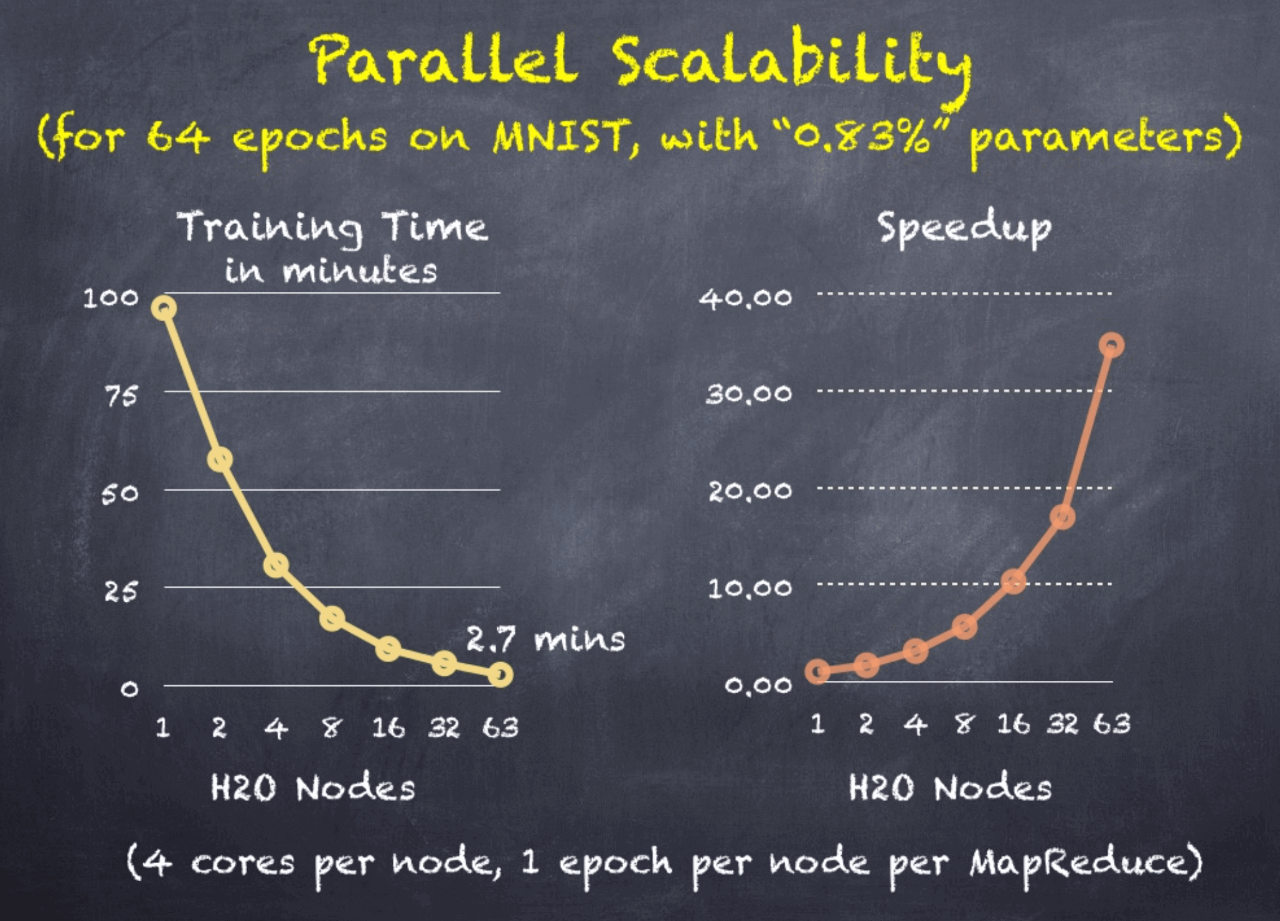
Without going into too much detail, the settings were a balance between fast convergence and high throughput. Also, the 1-node run had no communication overhead, while all the other runs had some communication overhead, so the comparison is not entirely fair, but more later!

Higgs Boson and H2O Deep Learning

Distributed H2O Deep Learning also achieved highly competitive results for the Higgs Boson dataset. It compares well to a recent Nature paper that used Deep Learning on GPUs to advance the frontier of particle physics.

Ebay Text Classification

For a successful application of distributed H2O Deep Learning for Ebay text classification with over 8500 columns and 580k rows, with hundreds of output classes, we refer to our Ebay Text Classification Slides.

Paypal Fraud Detection

Distributed H2O Deep Learning is used for Fraud Detection at PayPal.

Summary

H2O Deep Learning is a powerful, easy-to-use tool with highly competitive characteristics, both in terms of raw computing performance as well as predictive accuracy. H2O Deep Learning is used by customers in production. You can learn more about it from our H2O Deep Learning booklet or from H2O World Training, which will require only minimal changes to migrate from h2o to h2o-dev. For information about performance tuning of H2O Deep Learning, you really have to read this entire blog, it’s worth it!
Thank you for your interest! May H2O Deep Learning inspire you to build your own smart applications! We welcome your feedback!