
There’s a new major release of H2O, and it’s packed with new features and fixes! Among the big new features in this release, we’ve introduced the ability to define a Custom Loss Function in our GBM implementation, and we’ve extended the portfolio of our machine learning algorithms with the implementation of the SVM algorithm. The release is named after Shing-Tung Yau .
Custom Loss Function for GBM
In H2O, the GBM implementation of distributions and loss functions are tightly coupled. In the algorithm, a loss function is specified using the distribution parameter, and when specifying the distribution, the loss function is automatically selected as well.
Usually, the loss function is symmetric around a value. In some prediction problems, though, asymmetry in the loss function can improve results, for example, when we know that some kind of error is more undesirable than others (usually negative vs. positive error). We can use weights to cover some of these cases, but that is not suitable for more complicated calculations.
In H2O, you can upload a custom distribution and customize the loss function calculation. It is also possible to customize the whole distribution (select the link function, implement the calculation of initializing values, and change the gradient and gamma calculation) and to personalize the predefined distribution (Gaussian distribution for regression , Bernoulli distribution for binomial classification , and Multinomial distribution for multinomial classification) to customize loss function related functions only.
The documentation for custom distribution is available here . An example implementation of the asymmetric loss function on real data is available here .
SVM
Support-vector machine is an established supervised machine learning algorithm implemented by a number of software tools and libraries (one of the most popular being libsvm ). However, the SVM algorithm is challenging to implement in a scalable way so that it could be used on larger datasets and leverage the power of distributed systems. This version of H2O brings our users an implementation of the Parallel SVM (PSVM) algorithm that was designed in order to overcome the scalability issues of SVM and to address the bottlenecks of the traditional implementations. The main idea of the PSVM algorithm is to use a pre-processing step and reduce the amount of memory needed to hold the data by performing a row-based approximate matrix factorization. The PSVM algorithm makes a great fit for our map-reduce framework that internally H2O algorithms.
Our PSVM implementation can currently be used to solve binary classification problems using Radial Basis Function kernel. This complements the linear kernel SVM that H2O users already have available in Sparkling Water. The design of PSVM allows you to relatively easily include new kernel functions, and our users can thus expect to see support for different types of kernels as well as other new features in the coming versions of H2O.
For more details please refer to our documentation .
2D PDP
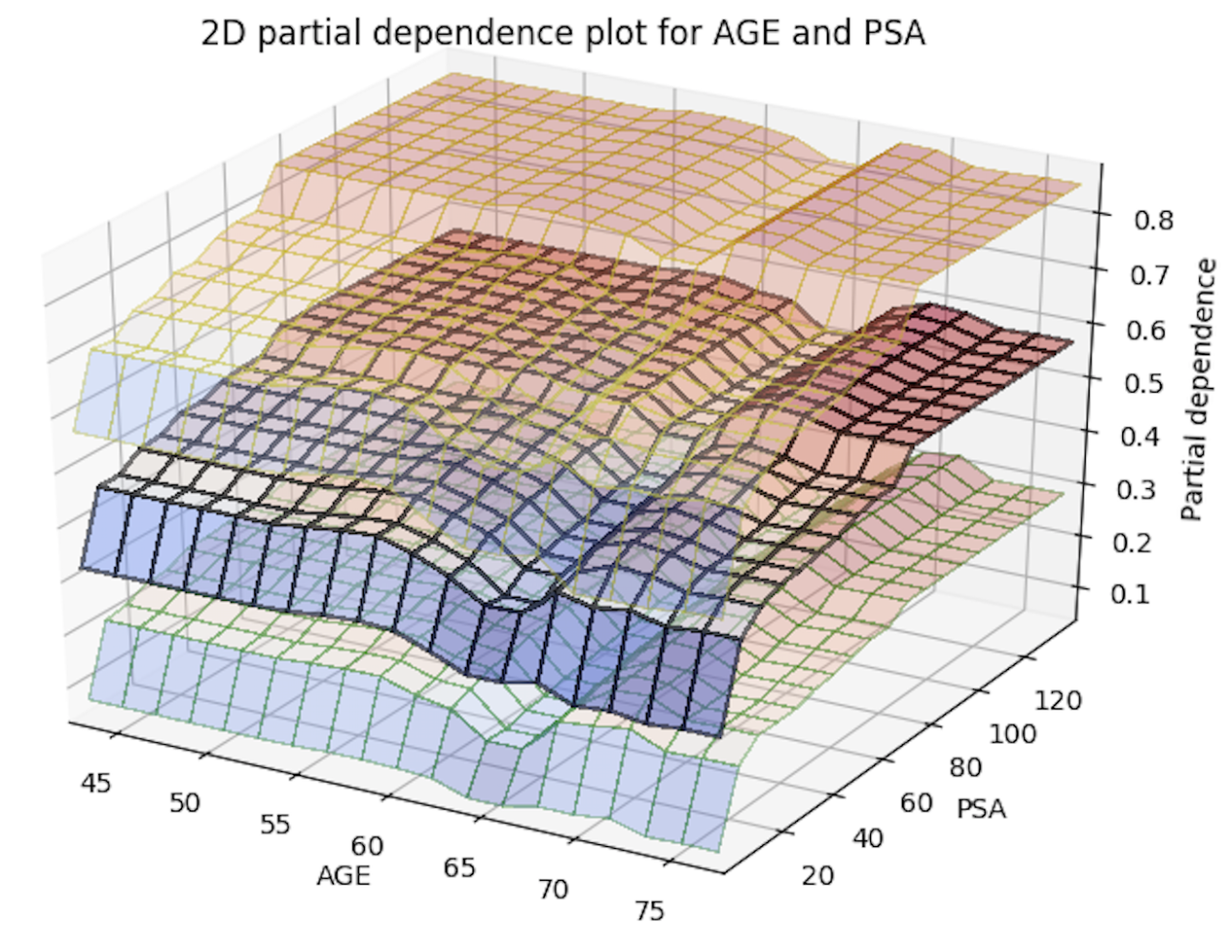
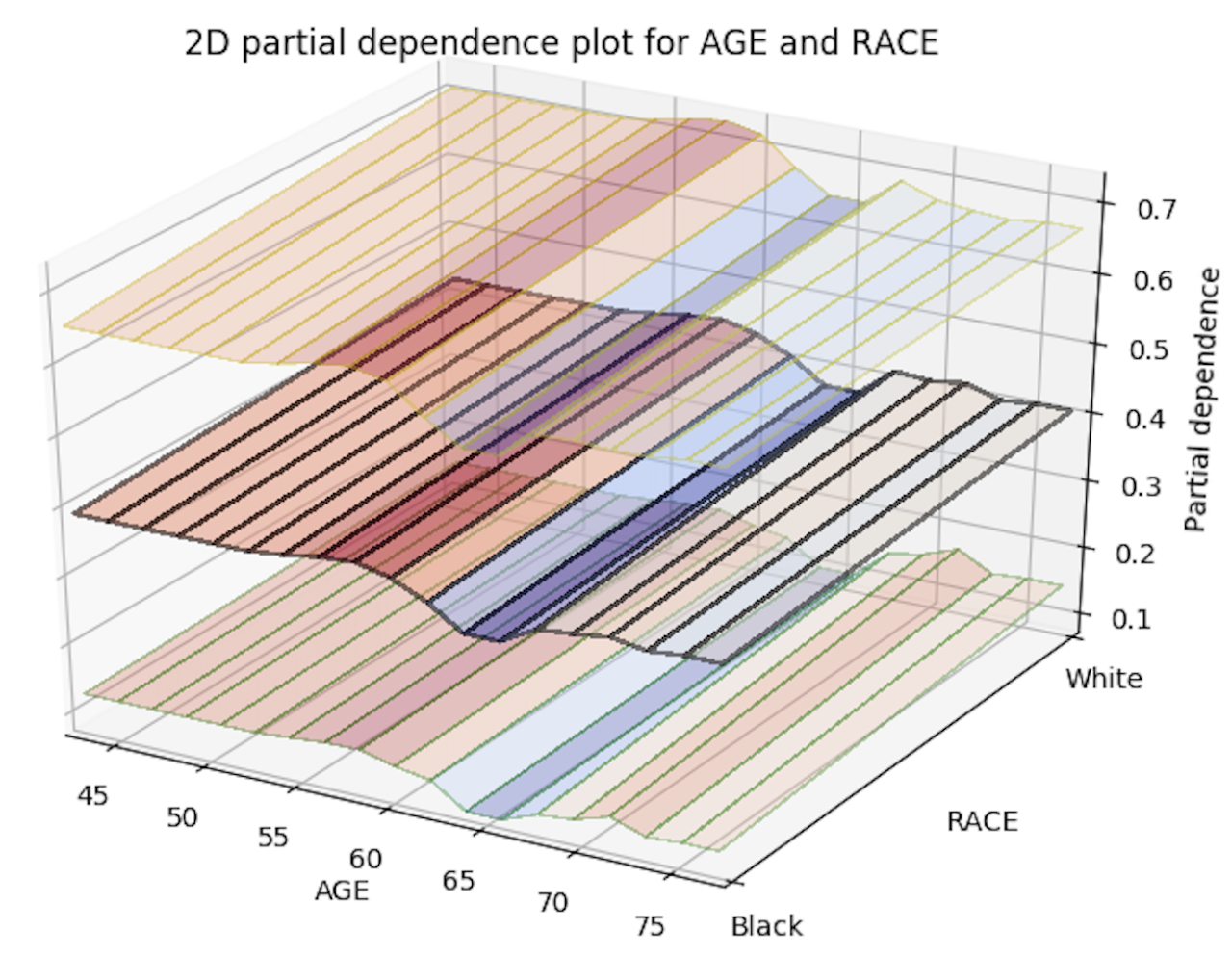
With this release, you can now generate 2D partial dependency plots with TWO variables instead of just one! The only thing you need to do to enable this is to add a new parameter, col_pairs_2dpdp, and fill it up with a list of variable pairs that you want to plot 2D partial plots with. For example, assume we have a prostate.csv dataset that we used to build a GBM model (called gbm_model), and we are interested in 1D partial plots for columns AGE, RACE, and DCAPS and 2D partial plots for variable pairs AGE, PSA and AGE, RACE. We can generate the 1D partial plots and 2D partial plots for gbm_model in Python using:
gbm_model.partial_plot(data = data, cols = [<style="color: #dd1144;">'AGE', <style="color: #dd1144;">'RACE', <style="color: #dd1144;">'DCAPS'],
 server = <style="color: #333333; font-weight: bold;">True, plot = <style="color: #333333; font-weight: bold;">True, user_splits = user_splits,
 col_pairs_2dpdp = [[<style="color: #dd1144;">'AGE', <style="color: #dd1144;">'PSA'],[<style="color: #dd1144;">'AGE', <style="color: #dd1144;">'RACE']],
 save_to_file = filename)
In R, you can make the same call using:
h2o.partialPlot(object = gbm_model, data = prostate_hex,
 cols = c(<style="color: #dd1144;">"RACE", <style="color: #dd1144;">"AGE”, “DCAPS"),
 col_pairs_2dpdp = list(c(<style="color: #dd1144;">"RACE", <style="color: #dd1144;">"AGE"), c(style="color: #dd1144;">"AGE", <style="color: #dd1144;">"PSA")),
 plot = TRUE, user_splits = user_splits_list,
 save_to = temp_filename_no_extension)
Below is an image of the 2D partial plots for the two variable pairs of interest:
Import MOJO with Metrics
The ability to re-import MOJOs into H2O and use them for scoring was introduced in version 3.24 (codename Yates). In the 3.26 release, we’ve enhanced the capabilities of the MOJO import API and made the MOJO models feel more like native H2O models by making the model information and metrics available. This functionality is useful for MOJO model inspection and evaluation. All MOJOs now receive the functionality to display basic model information and metrics:
- Basic model information (age, algorithm, description, scoring time, MSE, RMSE etc.)
- Training, validation and cross-validation metrics
- Cross-validation summary
More importantly, the Gradient Boosting Machine algorithm can now display model attributes exactly as a native H2O Model.
To inspect MOJO models, simply use the current means of model inspection in any available client (Python, R). This functionality fully integrates with the current functionality, and there are no changes to the API introduced by this functionality. If you’re new to MOJO import functionality, please refer to the MOJO Import documentation .
XGBoost Improvements
We are now using code equivalent to the latest stable release of XGBoost (0.82). This latest stable release brings performance improvements when running in OMP/CPU mode. We have also improved the way data is transferred from H2O to XGBoost Native memory. This process used to be single-threaded and was a big bottleneck especially for large data-sets. Now this process is fully parallelized, and users should see full CPU utilization during the entire XGBoost train process with much faster train times.
TreeSHAP for DRF
TreeShap was introduced for GBM and XGBoost in the 3.24.0.1 release of H2O. The 3.26.0.1 release of H2O now extends support for calculating SHAP (SHapley Additive exPlanation) values for Distributed Random Forest (DRF). SHAP values are consistent and locally accurate feature attribution values that can be used by a data scientist to understand and interpret the predictions of their model. H2O users will now be able to use the predict_contributions function to explain the predictions of their DRF model and visualize the explanation with the help of third party packages. Users will also be able to calculate the contributions for their DRF model deployed in their production environment, and this feature is also included for use in our model deployment package (MOJO).
An example of using H2O DRF to generate SHAP values is available here .
AutoML Improvements
We have a new feature in AutoML that allows users to view a detailed log of the events that happened during the AutoML run, including runtimes. The user can set three different levels of verbosity for the log using the verbosity parameter, and the information will appear as output during the AutoML run and also stored in the AutoML object to retrieve for further inspection after the run is complete. (See event_log and training_info AutoML object properties.)
Improvements to efficiency and memory use were also made to AutoML. Users can now delete AutoML objects (including all the models from an AutoML run) from memory, and models are now cleaned up properly if an AutoML job is cancelled. A bug affecting the reproducibility of the Random Forests in AutoML was also fixed.
Target Encoding MOJO support
Target encoding for Java API users was added to H2O-3 in 3.22.0.1. Since then, we also added support for R and Python clients. With the current release, we are just one step from MOJO support for Java API users. In 3.26.0.2, we will introduce the ability to generate a MOJO model for a target encoder so that it can be easily integrated into production pipelines. In a corresponding Sparkling Water release, integration with H2O-3 target encoding MOJO functionality will become available for users as well.
We will continue working on exposing MOJO support for target encoding in R/Py/Flow clients as well as on target encoding integration with AutoML.
Credits
This new H2O release is brought to you by Veronika Maurerova, Michal Kurka, Wendy Wong, Pavel Pscheidl, Jan Sterba, Navdeep Gill (special thanks!), Erin LeDell, Sebastien Poirier, and Andrey Spiridonov. We also thank Angela Bartz, Zain Haq, and Hannah Tillman as they have put tremendous effort into our documentation.