There’s a new major release of H2O, and it’s packed with new features and fixes! Among the big new features in this release, we’ve added RuleFit — an interpretable machine learning algorithm , introduced a new toolbox for model explainability, made Target Encoding work for all classes of problems, and integrated it in our AutoML  framework. On the technical side, we improved our Kubernetes integration, improved the performance of the platform, and further improved our XGBoost integration. The release is named after Ernst Zermelo .

New Algorithm: RuleFit

We are happy to add Rulefit to H2O. The Rulefit algorithm combines tree ensembles and linear models to take advantage of both methods: a tree ensemble’s accuracy and a linear model’s interpretability. The general algorithm fits a tree ensemble to the data, builds a rule ensemble by traversing each tree, evaluates the rules on the data to build a rule feature set, and fits a sparse linear model (LASSO) to the rule feature set joined with the original feature set.

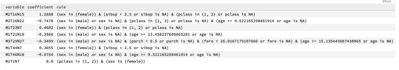
Since this is our first offering of the algorithm, a bunch of attractive features are still yet to be added. Stay tuned for more advanced diagnostic tools, extended support of tree ensembles to be used for rule generation, and further algorithm optimizations in the upcoming versions of H2O.

The documentation for Rulefit is available here .

Model Explainability

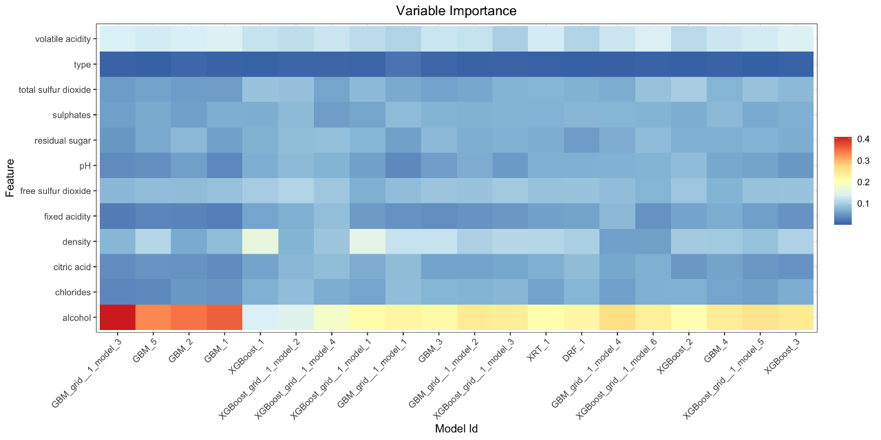
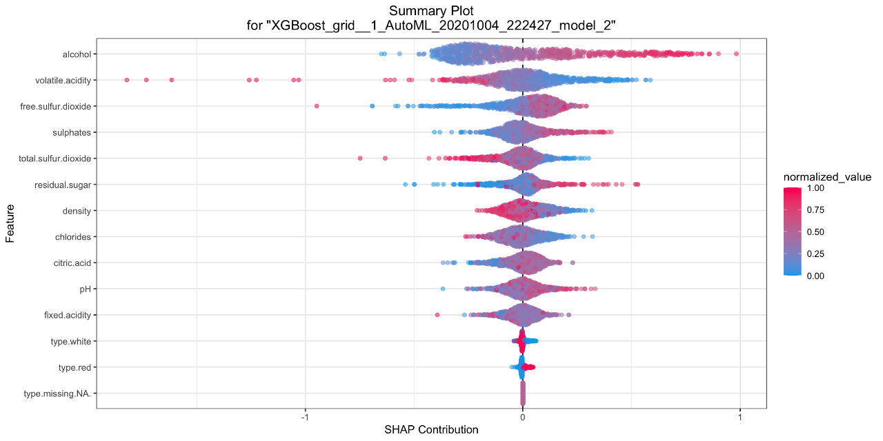
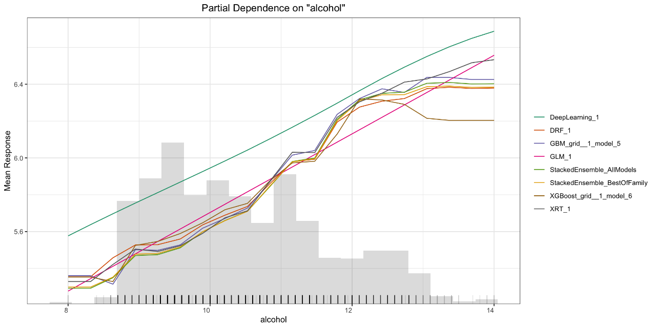
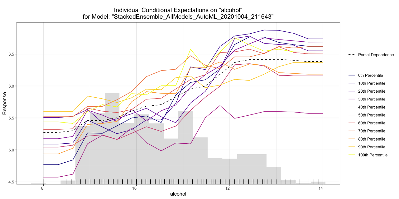
H2O now features a toolkit for Model Explainability. We provide a simple and automatic interface for a number of new and existing explainability methods and visualizations in H2O. The main functions, h2o.explain()  (for global explanations) and h2o.explain_row()  (for local explanations), work for individual H2O models, a list of models, or an H2O AutoML  object. The explain functions generate a list of explanations including individual units of explanation such as a partial dependence (PD) plot or a variable importance plot. Most of the explanations are visual, and the plots may be generated separately by individual utility functions (e.g. h2o.varimp_heatmap_plot() ). Here’s a list of what’s automatically generated for a list of models or an AutoML object:

• Leaderboard (compare all models)
• Confusion Matrix for Leader Model (classification only)
• Residual Analysis for Leader Model (regression only)
• Variable Importance of Top Base (non-Stacked) Model
• Variable Importance Heatmap (compare all non-Stacked models)
• Model Correlation Heatmap (compare all models)
• SHAP Summary of Top Tree-based Model (TreeSHAP)
• Partial Dependence (PD) Multi Plots (compare all models)
• Individual Conditional Expectation (ICE) Plots

Below are some examples of the visual explanations that will be automatically generated, in this case, by an AutoML object which contains a large number of models, as well as a “Leader Model.” Some visualizations explore groups of models (e.g. Variable Importance Heatmap, PD multi-plot), and some explore a single model (e.g. SHAP Summary plot, ICE plot). The documentation for Model Explainability, as well as visual examples for how all the plots are generated, is available here . We will continue to grow our explainability toolkit in future releases, and we’d love your feedback, so feel free to add your ideas and feature requests as comments on this ticket .

GAM Improvements

GAM models now offer full support for the traditional model productionizing tool – MOJO. The well-known download_mojo()  methods may now be used with GAM models.

Support has also been added for cross-validation  during GAM model training. Please set the nfolds  parameter on a GAM model to a value >= 2 to enable cross-validation.

Target Encoding for Regression and Multinomial Problems

Target Encoding is a powerful method for dealing with categorical variables, improving model performance, and avoiding overfitting. In this H2O release, we’ve also extended our existing Target Encoding support to include regression and multiclass classification problems. H2O’s target encoding can now be used for all classes of problems. In addition to that, we have also improved the API in order to make it easier to use and improve consistency in our client libraries (Python, R).

For more details about these updates, head over to the documentation page for Target Encoding . If you want to learn about the details of the API changes and their goals, you can read more in our Migration guide for Target Encoding .

XGBoost Improvements

We have updated XGBoost to the latest stable version (XGBoost 1.2.0). This upgrade brings in a bunch of performance improvements and bug-fixes. You can read more about this release in the XGBoost 1.2.0 release notes .

Our External XGBoost feature, where we are able to execute XGBoost models on a separate H2O cluster, has reached maturity. We have improved the performance of the initial data transfer between clusters which minimizes the performance differences between local and external XGBoost.

CoxPH Improvements

The main new feature in the CoxPH algorithm is the computation of the concordance index (also known as the concordance score). The concordance index rates the quality of a CoxPH model: if a perfect model orders events exactly the way they appear in the dataset, this score is 1; a CoxPH model which orders events randomly would score about 0.5; a model that orders events opposite to their order in a dataset would score 0.

If you have a CoxPH model (model ) and a data frame (data ) you can compute the score this way:

performance = model.model_performance(data)
concordance = performance.concordance()

Quantile and Tweedie Distribution for Monotone Constraints

Using monotone constraints in the Gradient Boosting Machine (GBM) algorithm in H2O-3 was previously limited to setting Gaussian and Bernoulli distributions. You can now improve your prediction by setting Tweedie and Quantile distributions, too. H2O-3 is the first library which supports Quantile distribution for monotone constraints.

When a new split is selected while tree building in GBM, every new subtree the column constraints during prediction have to be met. H2O-3 uses the histogram approach to select the best column split value, so the prediction in every node can easily be estimated during tree building. Then, the constraints are met during the construction of a tree. Monotone constraints can easily be implemented with Gaussian, Bernoulli, and Tweedie distributions because predictions are calculated directly from the leaves values of a tree.

On the contrary, because the Quantile distribution has the leaves values recalculated at the end of tree building using all the leaves prediction values, the monotone constraints are more difficult to implement. The prediction estimation can be more inaccurate for Quantile distribution than other distributions in every node during training because of the histogram values (this directly depends on the number of bins of histogram and the value of the quantile alpha).  The recalculation of leaves at the end of tree building also has to take constraints into account.

So, the result of the Quantile monotone constraint is the correct quantile prediction or the best updated possible quantile prediction with respect to the monotone constraint. For example, this feature can help define prediction intervals for regression problems using Gaussian distribution (see the image below).

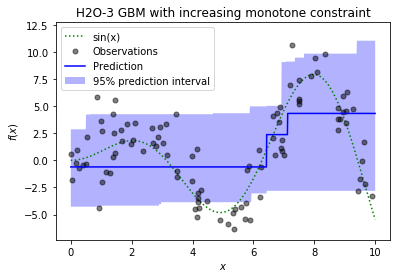
The Quantile monotone constraints demo is available here .

Precision-Recall Plot

Besides the Receiver operating characteristic curve (ROC) plot, the Precision-Recall plot is now available in H2O-3. Here is an example of how to get the plot and its resulting image:

perf = model.performance()
perf.plot(type="pr")

Helm Chart for H2O Kubernetes Deployments

Helm  can now be used to deploy H2O into a Kubernetes cluster. After the addition of the official H2O Helm repository to the local HELM registry, H2O can now be installed using helm.

helm repo add h2o https://charts.h2o.ai
helm install basic-h2o h2o/h2o-3
helm test basic-h2o

There are various settings and modifications available. To inspect the configuration options available, use the helm inspect values h2o/h2o  command.

For more information, check out this blog post .

AutoML Improvements

H2O AutoML  now features support for automatic Target Encoding , via the new preprocessing  parameter. In this first iteration, we have added a minimal Target Encoding integration which allows the user to turn on automatic Target Encoding (currently turned off by default). When activated, AutoML will automatically tune a Target Encoder model, and the transformations will be applied to all categorical columns (with >25 categories) for all of the tree-based algorithms inside AutoML (Random Forest, GBM and XGBoost). This is the beginning of an effort to improve performance of AutoML by focusing on feature transformations. Though we only support Target Encoding currently, the preprocessing  parameter will be extended in the future to include additional automatic data transformations. We also plan to allow customization of the preprocessing steps in a future release.

As noted in the Model Explainability section above, we now support automatic explanations for AutoML objects. This provides users greater insight into how the models generated through AutoML compare to each other across various dimensions, which can help you decide which model to deploy to production.

Credits

This new H2O release is brought to you by Zuzana Olajcova , Tomáš Frýda , Wendy Wong , Pavel Pscheidl , Sebastien Poirier , Jan Sterba , Ondřej Nekola , Veronika Maurerova , Erin LeDell , Michal Kurka , and Hannah Tillman .

H2O Training Center

Want to learn more about H2O? Check out our training center  for both self-paced tutorials and instructor-led courses.