
Standardized Coefficients

One of the (few) downsides of being in the Bay is the completely absurd traffic. Perhaps I am a bit more sensitive to this than most, given my epic daily commute. While I am normally inclined to whine about my cross-bay traverse a little, yesterday it paid off. You see, I’m used to making sense of things in my own way – which doesn’t always lend itself to clear explanation. Understanding something (or believing that I understand something, which is different) isn’t really where the rubber meets the road; when someone else asks me how something works it’s not really sufficient to say “isn’t it obvious?” or “it just does”. Aside from being a jerky thing to say, it’s not super productive. So when I had the experience of being completely unable to explain something to Tom for what seemed like an eon yesterday, I was a little disappointed in my own ability to communicate. So the totally long drive home was a good opportunity to consider this a bit extra.
At the heart was a discussion we were having about standardized coefficients. In GLM a standardized coefficient is a linear coefficient that has been expressed in terms of standard deviations rather than whatever the original units for that particular variable were. If that isn’t a clear explanation, you and Tom are on the same page, and I hope to do a better job now than I did yesterday, and rectify it by the end of this post.
If you use H2O to run our n=50 observations (which is like driving a Porsche where you should be driving a golf cart, but whatever…) this is the result:
Equation:
y = -34.7901*x[1] + -0.0666*x[2] + -0.0024*x[3] + 1336.4441*x[4] + 377.2923134309153
Our dependent variable (Y) is the annual consumption of gas (in millions of gallons)
| Gas Tax (cents/gallon) | -34.7901096 | -32.731014 |
|---|---|---|
| Average Annual Income (usd) | -0.06658840 | -37.796715 |
| Paved Highways (miles) | -0.00242587 | -8.38128406 |
| Drivers (proportion of pop. with DL) | 1336.4441156 | 73.3566276 |
| Intercept | 377.292313 | 576.7708333 |
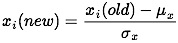
In keeping with our intuition about the world in general, when the price of gas goes up via taxes consumption goes down. The same directional relationship is true of average income and miles of paved highway, which is a bit less intuitive, but right now we don’t care. Not surprisingly, the density of drivers and gas consumption are positively related. Standardizing doesn’t change this; nor does it fundamentally change the way that a given x and y are correlated. So what’s changed? To get the standardized coefficient (SC) we transformed the values for each observation for that specific variable in the following way:
![]()
In English- we’ve mean centered and scaled by the standard deviation of that variable.
In the old coefficients we would say that a one cent increase in gas tax decreases the expected gas consumption by about 35 million gallons. In the standardized sense of the world we say that a one standard deviation increase in the gas tax decreases the expected gas consumption by about 33 million gallons.
At this point you might be going “ok, well, what did that get me? because there is practically no difference between one and the other.” And in this one, very narrow case, you would be right. In general, what you get is ease of interpretation, particularly when there is a big difference between the two, or when there is a large difference between the order of magnitude of the given x and y variables. Before we were trying to interpret the difference to the expected value of consumption imparted by a $1000 increase in average income, or a one mile increase in paved highway. Now you can think about impact in terms of where the relevant x value is for a particular observation with respect to the underlying distribution. A state that has a population that obtains drivers licenses at a rate higher (one standard deviation higher, in fact) than the national average will also consume 73 million gallons more on average.
Data notes:
Because I don’t particularly care to delve into some deep interpretation, nor do I wish to traumatize my still small audience, I decided to skip analyzing the most widely available on topic data – car accidents, injuries and fatalities. Instead we have super small text book data. You can procure a copy of your very own, along with the full citation information here: http://people.sc.fsu.edu/~jburkardt/datasets/regression/x15.txt